Manipulating data with R
Introducing R and RStudio
In today’s class we will process data using R, which is a very powerful tool, designed by statisticians for data analysis. Described on its website as “free software environment for statistical computing and graphics,” R is a programming language that opens a world of possibilities for making graphics and analyzing and processing data. Indeed, just about anything you may want to do with data can be done with R, from web scraping to making interactive graphics.
Next week we will make static graphics with R. We will explore’s its potential for making interactive charts and maps in week 13, and use it to make animations in week 14. Our goal for this week’s class is to get used to working with data in R.
RStudio is an “integrated development environment,” or IDE, for R that provides a user-friendly interface.
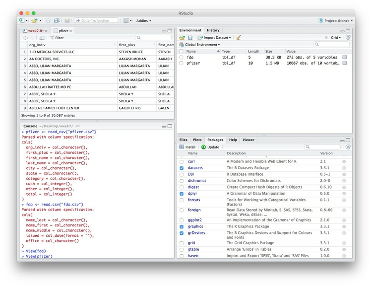
Launch RStudio, and the screen should look like this:
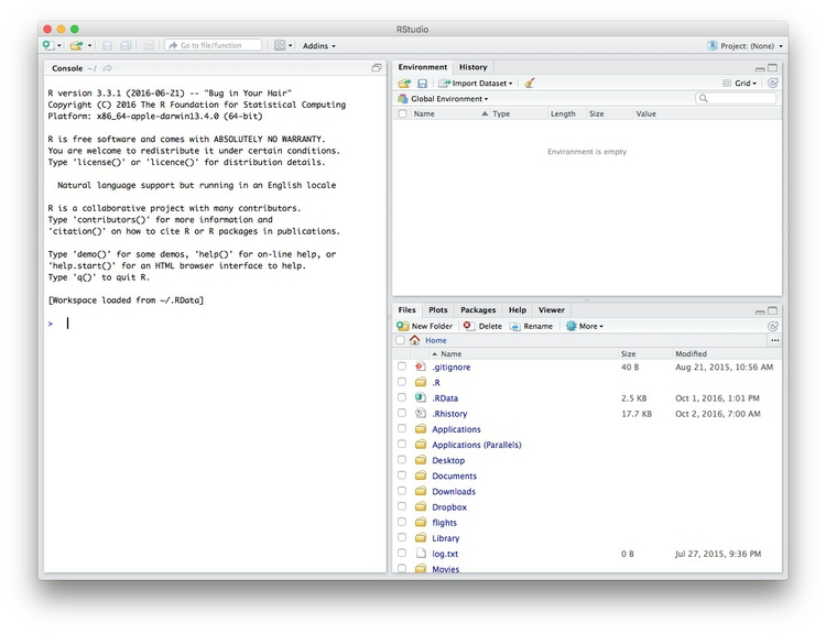
The main panel to the left is the R Console. Type valid R code into here, hit return, and it will be run. See what happens if you run:
print("Hello World!")
The data we will use today
Download the data for this session from here, unzip the folder and place it on your desktop. It contains the following files, used in reporting this story, which revealed that some of the doctors paid as “experts” by the drug company Pfizer had troubling disciplinary records:
pfizer.csvPayments made by Pfizer to doctors across the United States in the second half on 2009. Contains the following variables:org_indivFull name of the doctor, or their organization.first_plusDoctor’s first and middle names.first_namelast_name. First and last names.citystateCity and state.category of paymentType of payment, which includeExpert-led Forums, in which doctors lecture their peers on using Pfizer’s drugs, and `Professional Advising.cashValue of payments made in cash.otherValue of payments made in-kind, for example puschase of meals.totalvalue of payment, whether cash or in-kind.
fda.csvData on warning letters sent to doctors by the U.S. Food and Drug Administration, because of problems in the way in which they ran clinical trials testing experimental treatments. Contains the following variables:name_lastname_firstname_middleDoctor’s last, first, and middle names.issuedDate letter was sent.officeOffice within the FDA that sent the letter.
Reproducibility: Save your scripts
Data journalism should ideally be fully documented and reproducible. R makes this easy, as every operation performed can be saved in a script, and repeated by running that script. Click on the  icon at top left and select
 R Script. A new panel should now open:
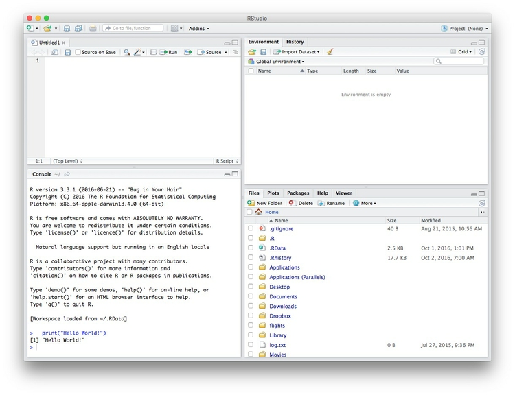
Any code we type in here can be run in the console. Hitting Run will run the line of code on which the cursor is sitting. To run multiple lines of code, highlight them and click Run.
Click on the save/disk icon in the script panel and save the blank script to the file on your desktop with the data for this week, calling it week7.R.
Set your working directory
Now we can set the working directory to this folder by selecting from the top menu Session>Set Working Directory>To Source File Location. (Doing so means we can load the files in this directory without having to refer to the full path for their location, and anything we save will be written to this folder.)
Notice how this code appears in the console:
setwd("~/Desktop/week7")
Save your data
The panel at top right has two tabs, the first showing the Environment, or all of the “objects” loaded into memory for this R session. We can save this as well, so we don’t have to load and process data again if we return to return to a project later.
(The second tab shows the History of the operations you have performed in RStudio.)
Click on the save/disk icon in the Environment panel to save and call the file week7.RData. You should see the following code appear in the Console:
save.image("~/Desktop/week7/week7.RData")
Copy this code into your script, placing it at the end, with a comment, explaining what it does:
# save session data
save.image("~/Desktop/week7/week7.RData")
Comment your code
Anything that appears on a line after # will be treated as a comment, and will be ignored when the code is run. Get into the habit of commenting your code: Don’t trust yourself to remember what it does!
Some R code basics
<-is known as an “assignment operator.” It means: “Make the object named to the left equal to the output of the code to the right.”&means AND, in Boolean logic, which we discussed in week 5 when working with web search forms.|means OR, in Boolean logic.!means NOT, in Boolean logic.- When referring to values entered as text, or to dates, put them in quote marks, like this:
"United States", or"2016-07-26". Numbers are not quoted. - When entering two or more values as a list, combine them using the function
c, with the values separated by commas, for example:c("2016-07-26","2016-08-04") - As in a spreadsheet, you can specify a range of values with a colon, for example:
c(1:10)creates a list of integers (whole numbers) from one to ten. Some common operators:
+-add, subtract.*/multiply, divide.><greater than, less than.>=<=greater than or equal to, less than or equal to.!=not equal to.
Equals signs can be a little confusing, but see how they are used in the code we use today:
==test whether an object is equal to a value. This is often used when filtering data, as we will see.=make an object equal to a value; works like<-, but used within the brackets of a function.
We encountered functions in week 1 in the context of spreadsheet formulas. They are followed by brackets, and act on the code in the brackets.
Important: Object and variable names in R should not contain spaces.
Install and load R packages
Much of the power of R comes from the thousands of “packages” written by its community of open source contributors. These are optimized for specific statistical, graphical or data-processing tasks. To see what packages are available in the basic distribution of R, select the Packages tab in the panel at bottom right. To find packages for particular tasks, try searching Google using appropriate keywords and the phrase “R package.”
In this class, we will work with two incredibly useful packages developed by Hadley Wickham, chief scientist at RStudio:
These and several other useful packages have been combined into a super-package called tidyverse.
To install a package, click on the Install icon in the Packages tab, type its name into the dialog box, and make sure that Install dependencies is checked, as some packages will only run correctly if other packages are also installed. Click Install and all of the required packages should install:
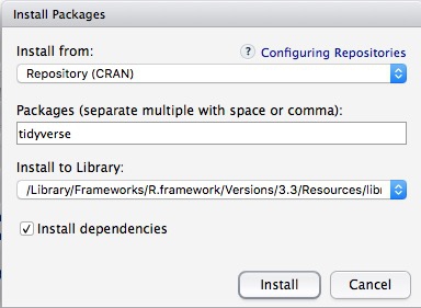
Notice that the following code appears in the console:
install.packages("tidyverse")
So you can also install packages with cod in this format, without using the point-and-click interface.
Each time you start R, it’s a good idea to click on Update in the Packages panel to update all your installed packages to the latest versions.
Installing a package makes it available to you, but to use it in any R session you need to load it. You can do this by checking its box in the Packages tab. However, we will enter the following code into our script, then highlight these lines of code and run them:
# load packages to read, write and manipulate data
library(readr)
library(dplyr)
At this point, and at regular intervals, save your script, by clicking the save/disk icon in the script panel, or using the ⌘-S keyboard shortcut.
Load and view data
Load data
You can load data into the current R session by selecting Import Dataset>From Text File... in the Environment tab.
However, we will use the read_csv function from the readr package. Copy the following code into your script and Run:
# load data of pfizer payments to doctors and warning letters sent by food and drug adminstration
pfizer <- read_csv("pfizer.csv")
fda <- read_csv("fda.csv")
Notice that the Environment now contains two objects, of the type tbl_df, a variety of the standard R object for holding tables of data, known as a data frame:
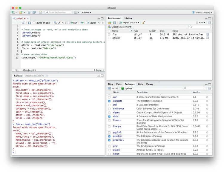
The Value for each data frame details the number of columns, and the number of rows, or observations, in the data.
You can remove any object from your environment by checking it in the Grid view and clicking the broom icon.
Examine the data
We can View data at any time by clicking on its table icon in the Environment tab in the Grid view.
Here, for example, I am looking at the pfizer view:
The str function will tell you more about the columns in your data, including their data type. Copy this code into your script and Run:
# view structure of data
str(pfizer)
This should give the following output in the R Console:
Classes ‘tbl_df’, ‘tbl’ and 'data.frame':    10087 obs. of  10 variables:
 $ org_indiv : chr  "3-D MEDICAL SERVICES LLC" "AA DOCTORS, INC." "ABBO, LILIAN MARGARITA" "ABBO, LILIAN MARGARITA" ...
 $ first_plus: chr  "STEVEN BRUCE" "AAKASH MOHAN" "LILIAN MARGARITA" "LILIAN MARGARITA" ...
 $ first_name: chr  "STEVEN" "AAKASH" "LILIAN" "LILIAN" ...
 $ last_name : chr  "DEITELZWEIG" "AHUJA" "ABBO" "ABBO" ...
 $ city      : chr  "NEW ORLEANS" "PASO ROBLES" "MIAMI" "MIAMI" ...
 $ state     : chr  "LA" "CA" "FL" "FL" ...
 $ category  : chr  "Professional Advising" "Expert-Led Forums" "Business Related Travel" "Meals" ...
 $ cash      : int  2625 1000 0 0 1800 750 0 825 3000 0 ...
 $ other     : int  0 0 448 119 0 0 47 0 0 396 ...
 $ total     : int  2625 1000 448 119 1800 750 47 825 3000 396 ...
chr means “character,” or a string of text (which can be treated as a categorical variable); int means an integer, or whole number.
Also examine the structure of the fda data frame using the following code:
str(fda)
This should be the console output:
Classes ‘tbl_df’, ‘tbl’ and 'data.frame':    272 obs. of  5 variables:
 $ name_last  : chr  "ADELGLASS" "ADKINSON" "ALLEN" "AMSTERDAM" ...
 $ name_first : chr  "JEFFREY" "N." "MARK" "DANIEL" ...
 $ name_middle: chr  "M." "FRANKLIN" "S." NA ...
 $ issued     : Date, format: "1999-05-25" ...
 $ office     : chr  "Center for Drug Evaluation and Research" "Center for Biologics Evaluation and Research" "Center for Devices and Radiological Health" "Center for Biologics Evaluation and Research" ...
Notice that issued has been recognized as a Date variable. Other common data types include num, for numbers that may contain decimals and POSIXct for full date and time.
If you run into any trouble importing data with readr, you may need to specify the data types for some columns — in particular for date and time. This link explains how to set data types for individual variables when importing data with readr.
To specify an individual column use the name of the data frame and the column name, separated by $. Type this into your script and run:
# print values for total in pfizer data
pfizer$total
The output will be the first 10,000 values for that column.
If you need to change the data type for any column, use the following functions:
as.characterconverts to a text string.as.numericconverts to a number.as.factorconverts to a categorical variable.as.integerconverts to an integeras.Dateconverts to a dateas.POSIXctconvets to a full date and time.
(Conversions to full dates and times can get complicated, because of timezones. Contact me for advice if you need to work with full dates and times for your project!)
Now add the following code to your script to convert the convert total in the pfizer data to a numeric variable (which would allow it to hold decimal values, if we had any).
# convert total to numeric variable
pfizer$total <- as.numeric(pfizer$total)
str(pfizer)
Notice that the data type for total has now changed:
Classes ‘tbl_df’, ‘tbl’ and 'data.frame':    10087 obs. of  10 variables:
 $ org_indiv : chr  "3-D MEDICAL SERVICES LLC" "AA DOCTORS, INC." "ABBO, LILIAN MARGARITA" "ABBO, LILIAN MARGARITA" ...
 $ first_plus: chr  "STEVEN BRUCE" "AAKASH MOHAN" "LILIAN MARGARITA" "LILIAN MARGARITA" ...
 $ first_name: chr  "STEVEN" "AAKASH" "LILIAN" "LILIAN" ...
 $ last_name : chr  "DEITELZWEIG" "AHUJA" "ABBO" "ABBO" ...
 $ city      : chr  "NEW ORLEANS" "PASO ROBLES" "MIAMI" "MIAMI" ...
 $ state     : chr  "LA" "CA" "FL" "FL" ...
 $ category  : chr  "Professional Advising" "Expert-Led Forums" "Business Related Travel" "Meals" ...
 $ cash      : int  2625 1000 0 0 1800 750 0 825 3000 0 ...
 $ other     : int  0 0 448 119 0 0 47 0 0 396 ...
 $ total     : num  2625 1000 448 119 1800 ...
The summary function will run a quick statistical summary of a data frame, calculating mean, median and quartile values for continuous variables:
# summary of pfizer data
summary(pfizer)
Here is the last part of the console output:
     total
 Min.   :      0
 1st Qu.:    191
 Median :    750
 Mean   :   3507
 3rd Qu.:   2000
 Max.   :1185466
Manipulate and analyze data
Now we will use dplyr to manipulate the data, using the basic operations we discussed in week 1:
Sort: Largest to smallest, oldest to newest, alphabetical etc.
Filter: Select a defined subset of the data.
Summarize/Aggregate: Deriving one value from a series of other values to produce a summary statistic. Examples include: count, sum, mean, median, maximum, minimum etc. Often you’ll group data into categories first, and then aggregate by group.
Join: Merging entries from two or more datasets based on common field(s), e.g. unique ID number, last name and first name.
Here are some of the most useful functions in dplyr:
selectChoose which columns to include.filterFilter the data.arrangeSort the data, by size for continuous variables, by date, or alphabetically.group_byGroup the data by a categorical variable.summarizeSummarize, or aggregate (for each group if followinggroup_by). Often used in conjunction with functions including:meanCalculate the mean, or average.medianCalculate the median.maxFind the maximum value.minFind the minimum valuesumAdd all the values together.nCount the number of records.
mutateCreate new column(s) in the data, or change existing column(s).renameRename column(s).bind_rowsMerge two data frames into one, combining data from columns with the same name.
There are also various functions to join data, which we will explore below.
These functions can be chained together using the operator %>% which makes the output of one line of code the input for the next. This allows you to run through a series of operations in logical order. I find it helpful to think of %>% as “then.”
Filter and sort data
Now we will filter and sort the data in specific ways. For each of the following examples, copy the code that follows into your script, and view the results. Notice how we create a new objects to hold the processed data.
Find doctors in California paid $10,000 or more by Pfizer to run “Expert-Led Forums.”
# doctors in California who were paid $10,000 or more by Pfizer to run “Expert-Led Forums.”
ca_expert_10000 <- pfizer %>%
  filter(state == "CA" & total >= 10000 & category == "Expert-Led Forums")
Notice the use of == to find values that match the specified text, >= for greater than or equal to, and the Boolean operator &.
Now add a sort to the end of the code to list the doctors in descending order by the payments received:
# doctors in California who were paid $10,000 or more by Pfizer to run “Expert-Led Forums.”
ca_expert_10000 <- pfizer %>%
  filter(state == "CA" & total >= 10000 & category == "Expert-Led Forums") %>%
  arrange(desc(total))
If you arrange without the desc function, the sort will be from smallest to largest.
Find doctors in California or New York who were paid $10,000 or more by Pfizer to run “Expert-Led Forums.”
ca_ny_expert_10000 <- pfizer %>%
  filter((state == "CA" | state == "NY") & total >= 10000 & category == "Expert-Led Forums") %>%
  arrange(desc(total))
Notice the use of the | Boolean operator, and the brackets around that part of the query. This ensures that this part of the query is run first. See what happens if you exclude them.
Find doctors in states other than California who were paid $10,000 or more by Pfizer to run “Expert-Led Forums.”
not_ca_expert_10000 <- pfizer %>%
  filter(state != "CA" & total >= 10000 & category=="Expert-Led Forums")) %>%
  arrange(desc(total))
Notice the use of the != operator to exclude doctors in California.
Find the 20 doctors across the four largest states (CA, TX, FL, NY) who were paid the most for professional advice.
ca_ny_tx_fl_prof_top20 <- pfizer %>%
  filter((state=="CA" | state == "NY" | state == "TX" | state == "FL") & category == "Professional Advising") %>%
  arrange(desc(total)) %>%
  head(20)
Notice the use of head, which grabs a defined number of rows from the start of a data frame. Here, it is crucial to run the sort first! See what happens if you change the order of the last two lines.
Filter the data for all payments for running Expert-Led Forums or for Professional Advising, and arrange alphabetically by doctor (last name, then first name)
# Filter the data for all payments for running Expert-Led Forums or for Professional Advising, and arrange alphabetically by doctor (last name, then first name)
expert_advice <- pfizer %>%
  filter(category == "Expert-Led Forums" | category == "Professional Advising") %>%
  arrange(last_name, first_name)
Notice that you can sort by multiple variables, separated by commas.
Use pattern matching to filter text
The following code uses the grepl function to find values containing a particular string of text. This can simplify the code used to filter based on text.
# use pattern matching to filter text
expert_advice <- pfizer %>%
  filter(grepl("Expert|Professional", category)) %>%
  arrange(last_name, first_name)

not_expert_advice <- pfizer %>%
  filter(!grepl("Expert|Professional", category)) %>%
  arrange(last_name, first_name)
This code differs only by the ! Boolean operator. Notice that it has split the data into two, based on categories of payment.
Append one data frame to another
The following code uses the bind_rows function to append one data frame to another, here recreating the unfiltered data from the two data frames above.
# merge/append data frames
pfizer2 <- bind_rows(expert_advice, not_expert_advice)
Write data to a CSV file
readr can write data to CSV and other text files.
# write expert_advice data to a csv file
write_csv(expert_advice, "expert_advice.csv", na="")
When you run this code, a CSV file with the data should be saved in your week7 folder. na="" ensures that any empty cells in the data frame are saved as blanks — R represents null values as NA, so if you don’t include this, any null values will appear as NA in the saved file.
Group and summarize data
Calculate the total payments, by state
# calculate total payments by state
state_sum <- pfizer %>%
  group_by(state) %>%
  summarize(sum = sum(total)) %>%
  arrange(desc(sum))
Notice the use of group_by followed by summarize to group and summarize data, here using the function sum.
Calculate some additional summary statistics, by state
# As above, but for each state also calculate the median payment, and the number of payments
state_summary <- pfizer %>%
  group_by(state) %>%
  summarize(sum = sum(total), median = median(total), count = n()) %>%
  arrange(desc(sum))
Notice the use of multiple summary functions, sum, median, and n. (You don’t specify a variable for n because it is simply counting the number of rows in the data.)
Group and summarize for multiple categories
# as above, but group by state and category
state_category_summary <- pfizer %>%
  group_by(state, category) %>%
  summarize(sum = sum(total), median = median(total), count = n()) %>%
  arrange(state, category)
As for arrange, you can group_by by multiple variables, separated by commas.
Working with dates
Now let’s run see how to work with dates, using the FDA warning letters data.
Filter the data for letters sent from the start of 2005 onwards
# FDA warning letters sent from the start of 2005 onwards
post2005 <- fda %>%
  filter(issued >= "2005-01-01") %>%
  arrange(issued)
Notice that operators like >= can be used for dates, as well as for numbers.
Count the number of letters issued by year
# count the letters by year
letters_year <- fda %>%
  mutate(year = format(issued, "%Y")) %>%
  group_by(year) %>%
  summarize(letters=n())
This code introduces dplyr’s mutate function to create a new column in the data. The new variable year is the four-digit year "%Y (see here for more on time and date formats in R), extracted from the issued dates using the format function. Then the code groups by year and counts the number of letters for each one.
Add columns giving the number of days and weeks that have elapsed since each letter was sent
# add new columns showing many days and weeks elapsed since each letter was sent
fda <- fda %>%
  mutate(days_elapsed = Sys.Date() - issued,
          weeks_elapsed = difftime(Sys.Date(), issued, units = "weeks"))
Notice in the first line that this code changes the fda data frame, rather than creating a new object. The function Sys.Date returns the current date, and if you subtract another date, it will calculate the difference in days. To calculate date and time differences using other units, use the difftime function.
Notice also that you can mutate multiple columns at one go, separated by commas.
Join data from two data frames
There are also a number of join functions in dplyr to combine data from two data frames. Here are the most useful:
inner_join()returns values from both tables only where there is a match.left_join()returns all the values from the first-mentioned table, plus those from the second table that match.semi_join()filters the first-mentioned table to include only values that have matches in the second table.anti_join()filters the first-mentioned table to include only values that have no matches in the second table.
To illustrate, these joins will find doctors paid by Pfizer to run expert led forums who had also received a warning letter from the FDA:
# join to identify doctors paid to run Expert-led forums who also received a warning letter
expert_warned_inner <- inner_join(pfizer, fda, by=c("first_name" = "name_first", "last_name" = "name_last")) %>%
  filter(category=="Expert-Led Forums")

expert_warned_semi <- semi_join(pfizer, fda, by=c("first_name" = "name_first", "last_name" = "name_last")) %>%
  filter(category=="Expert-Led Forums")
The code in by=c() defines how the join should be made. If instructions on how to join the tables are not supplied, dplyr will look for columns with matching names, and perform the join based on those.
The difference between the two joins above is that the first contains all of the columns from both data frames, while the second gives only columns from the pfizer data frame.
In practice, you may wish to inner_join and then use dplyr’s select function to select the columns that you want to retain, for example:
# as above, but select desired columns from data
expert_warned <- inner_join(pfizer, fda, by=c("first_name" = "name_first", "last_name" = "name_last")) %>%
  filter(category=="Expert-Led Forums") %>%
  select(first_plus, last_name, city, state, total, issued)

expert_warned <- inner_join(pfizer, fda, by=c("first_name" = "name_first", "last_name" = "name_last")) %>%
  filter(category=="Expert-Led Forums") %>%
  select(2:5,10,12)
Notice that you can select by columns’ names, or by their positions, where 1 is the first column, 3 is the third, and so on.
Here is a useful reference for managing joins with dplyr.
Further reading
RStudio Data Wrangling Cheet Sheet
Also introduces the tidyr package, which can manage wide-to-long transformations, among other data manipulations.
Stack Overflow
For any work involving code, this question-and-answer site is a great resource for when you get stuck, to see how others have solved similar problems. Search the site, or browse R questions